menguji perbedaan variasi antar kelompok (lebih dari 2) variabel yang akan kita uji
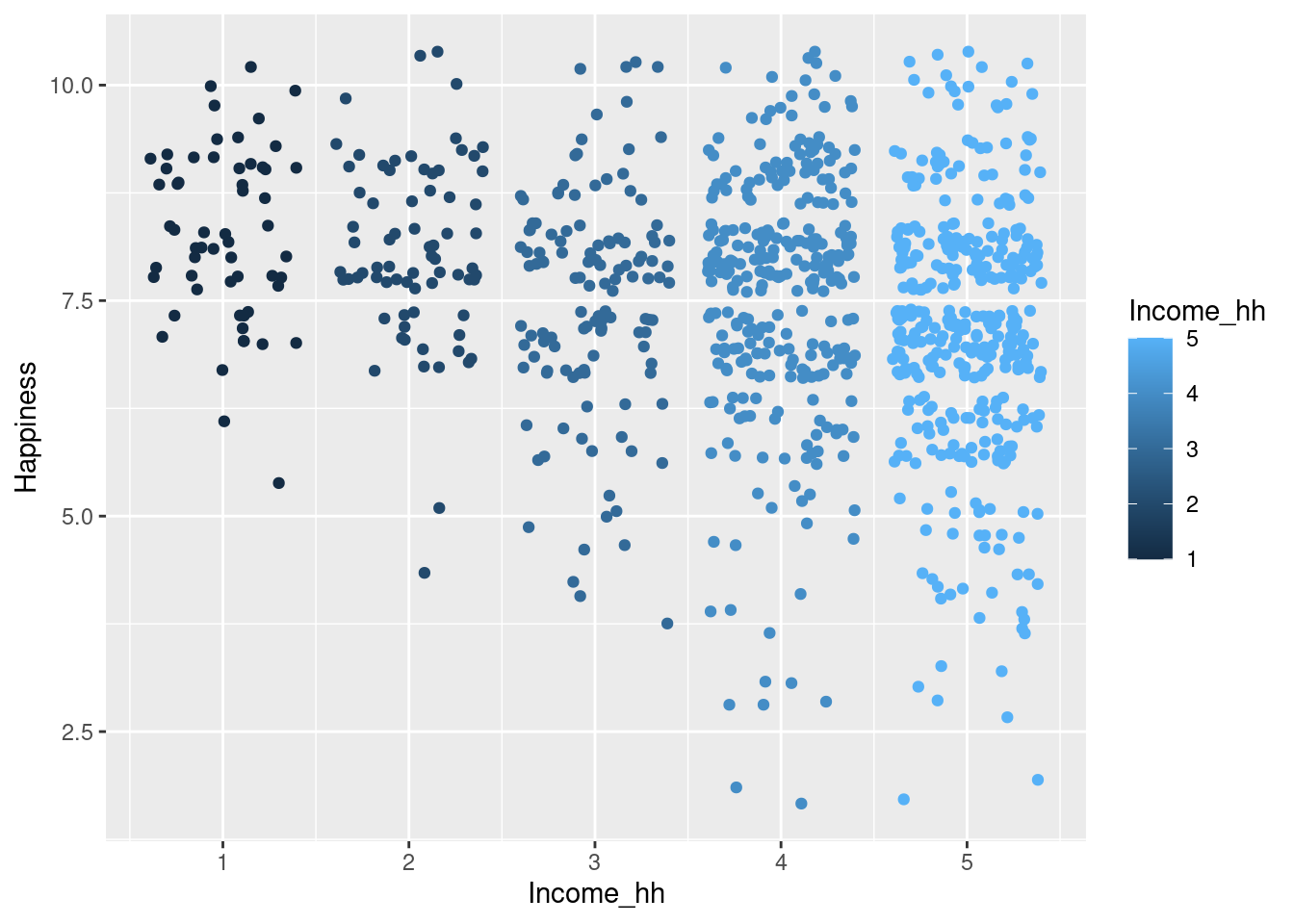
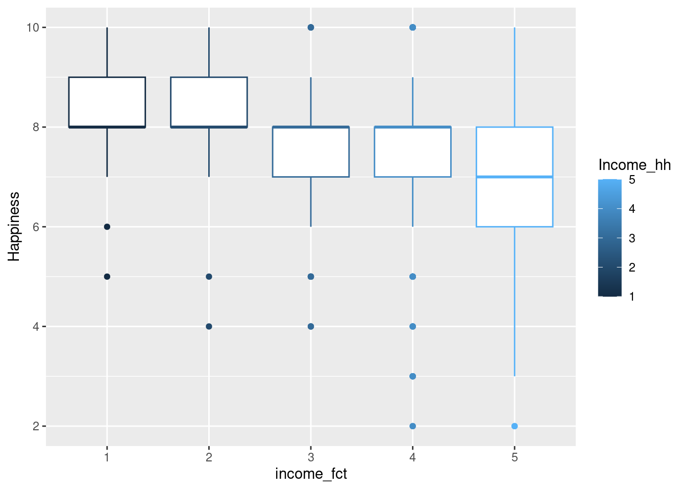
kita akan menguji household income and happiness
RQ: apakah terdapat perbedaan tingkat kebahagiaan ditinjau dari tingkat pendapatan?
6.2 Library
library(psych)library(tidyverse)
── Attaching core tidyverse packages ──────────────────────── tidyverse 2.0.0 ──
✔ dplyr     1.1.1     ✔ readr     2.1.4
✔ forcats   1.0.0     ✔ stringr   1.5.0
✔ ggplot2   3.4.2     ✔ tibble    3.2.1
✔ lubridate 1.9.2     ✔ tidyr     1.3.0
✔ purrr     1.0.1
── Conflicts ────────────────────────────────────────── tidyverse_conflicts() ──
✖ ggplot2::%+%()   masks psych::%+%()
✖ ggplot2::alpha() masks psych::alpha()
✖ dplyr::filter()  masks stats::filter()
✖ dplyr::lag()     masks stats::lag()
ℹ Use the conflicted package (<http://conflicted.r-lib.org/>) to force all conflicts to become errors
library(rstatix)
Attaching package: 'rstatix'

The following object is masked from 'package:stats':

    filter
library(report)
6.3 Membaca data
data pengukuran tingkat kebahagiaan
tingkat DIY
income <-read_csv("income_happiness_diy.csv")
Rows: 913 Columns: 4
── Column specification ────────────────────────────────────────────────────────
Delimiter: ","
chr (1): Provinsi
dbl (3): Income_ind, Income_hh, Happiness

ℹ Use `spec()` to retrieve the full column specification for this data.
ℹ Specify the column types or set `show_col_types = FALSE` to quiet this message.
beda <-aov(Happiness~Income_hh, data=income)summary(beda)
             Df Sum Sq Mean Sq F value   Pr(>F)
Income_hh     1   87.2   87.24   45.71 2.45e-11 ***
Residuals   911 1738.8    1.91
---
Signif. codes:  0 '***' 0.001 '**' 0.01 '*' 0.05 '.' 0.1 ' ' 1
6.8 Effect Size
A small effect size is about .01.
A medium effect size is about .06.
A large effect size is about .14.
report(beda)
The ANOVA (formula: Happiness ~ Income_hh) suggests that:

  - The main effect of Income_hh is statistically significant and small (F(1,
911) = 45.71, p < .001; Eta2 = 0.05, 95% CI [0.03, 1.00])

Effect sizes were labelled following Field's (2013) recommendations.